Introduction
In this tutorial, you will learn about working with data in R. In particular, this tutorial will cover importing data from various file types into R including:
- csv files
- Excel files
- R data files
Files and File Structures
Files on your local computer
When you are working in R on your local computer and you want to import a data file into your R session for an analysis, you will need to tell R where it can find the data file. This is why I suggested creating a ‘Data’ folder in your class folder. If you save all of the data files for this class in that folder, you can always use the same general syntax for telling R where your file is.
For this tutorial, we are working on the web, so R doesn’t have access to the local files on your device. I have included all of the data files we will be using in this tutorial on a webpage that we can access online. You may need to change this code slightly to when running code for your assignments in this class to work with your computer’s file structure.
Checking your working directory
One good idea when you start working on a new analysis is to make sure you know where within your computer’s file structure you are working so you can figure out how to access various files.
We can use the function getwd() to have R print out the path to the directory (folder) we are currently working in.
Try running the code in this block:
You should see the output is:
“/home/web_user”
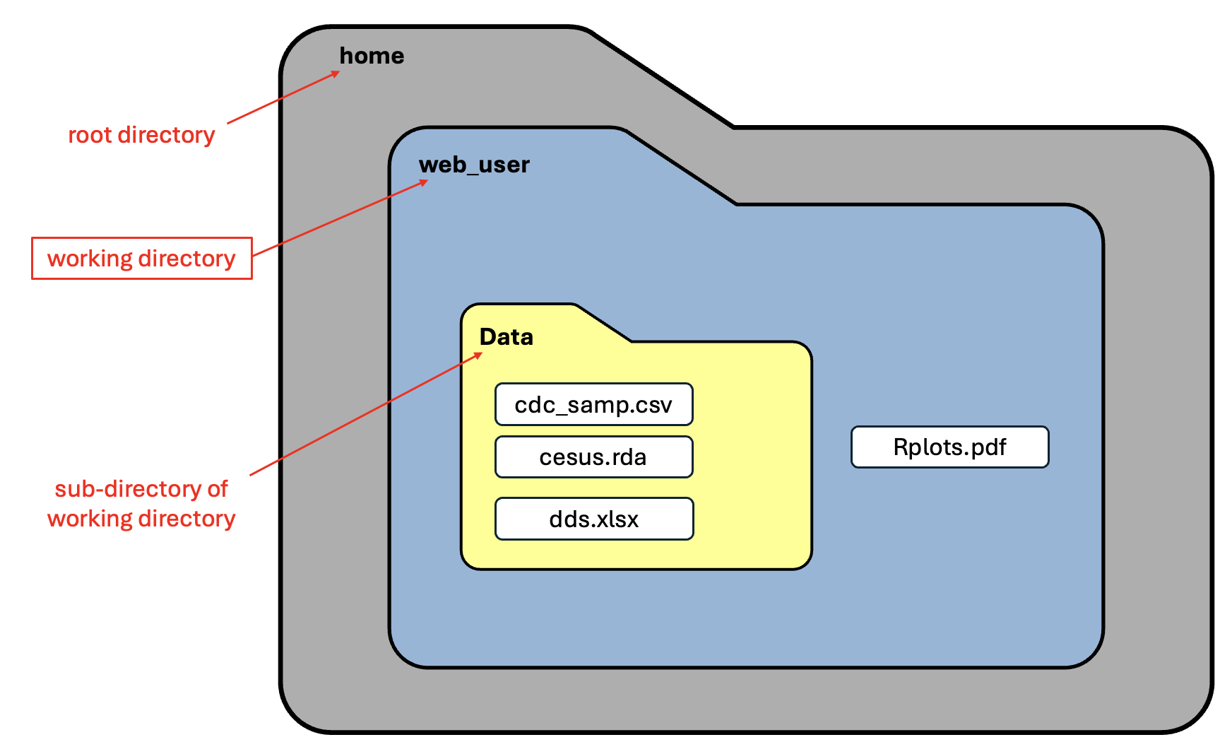
This is because we are working in R on the web. This is telling us that we are in a sub-directory of the “home” directory called “web_user”. That is, “web_user” is a directory (folder) inside the larger directory (folder) called “home”. You read file paths from left to right.
Try running this in your Console in RStudio on your computer, and you should see a file path that corresponds to the file structure on your computer.
File paths
File paths are a way of specifying the location of a file within a computer’s file system. There are two kinds of file paths, absolute paths and relative paths. Both can be useful in different situations.
Absolute file paths are file paths that start at the root node of your computer (often starting with something like “C:” in Windows and “/Users/” in Unix-like operating systems like macOS). Absolute paths can get fairly long if files are contained within many levels of sub-directories.
Relative file paths are paths that start at the current working directory, and are therefore often shorter than absolute paths.
The function we used above, getwd(), prints absolute paths, so we are currently working in the “web_user” sub-directory of the root directory called “home”. The image below is a visual representation of the file structure.
List files in working directory
To check the files that exist in our current directory, we can use the function list.files() to print a list of all the files that are stored in the directory where we are currently working. If we just want to print the files in our working directory, we can run the function without giving it a file path and just leave the inside of the parentheses blank (this will assume you want to list the files in your current directory). We could also input a file path to the function.
Try running the code in this block:
The output should look something like this:
[1] “Data” “Rplots.pdf”
This tells us that there are 2 objects that we have access to in this directory:
- A folder called “Data”
- One clue that it’s a folder instead of a file is that it doesn’t have a file extension (like “.pdf”) on the end
- A file called “Rplots.pdf”
- We won’t be working with this file
If we want to see the files contained within the sub-folder “Data”, we can add this to the end of our absolute file path within the path argument:
Alternatively, we could add an extra argument to the original code that allows us to print files within subdirectories recursively. This argument tells R to print the contents of any subfolders contained within our directory (stopping when there are no further nested folders).
All of these tell us that within the sub-folder called “Data”, we have three files:
- a file called “cdc_samp.csv”
- a file called “census.rda”
- a file called “dds.xlsx”
These are the data files that we will be working with in this tutorial.
Types of Files
The main types of files that we will work with in this class are:
| File Type | Description | File Extension |
|---|---|---|
| CSV files | This stands for “comma separated value”. These are files that have rows with entries separated by commas to indicate the different columns | .csv |
| Excel files | Files in Excel workbook/sheet format | .xls or .xlsx |
| R data files | Files with saved R objects | .RData or .rda |
The three files we will use today have the following names:
- “cdc_samp.csv” : a csv file with demographic data from the CDC
- “dds.xlsx” : an Excel file with data from the Department of Disability Services in California
- “census.rda”: an R data file with data from the US Census Bureau
Importing Data
Importing a csv file
To import a csv file to R, we can use the function read.csv(). There is a similar function in the tidyverse package called read_csv() that we can also use. We’ll go ahead and use the tidyverse version.
The syntax to use this function is:
name_for_data = read_csv("path_to_data")
Here
name_for_datais any name you choose to call the data frame object that you will be creating with theread_csv()function. It can be helpful to give it a name that is relevant to the data, but you can call it whatever you want (with some limits–for example, the name can’t start with a number)."path_to_data"is the file path that will tell R where to look for your data. You can either provide the function with an absolute path to the file (starting with the root directory of your computer) or a relative path, starting at the current working directory.
Warning: Naming the object is very important!
If you forget to choose a name for your data frame, R will import the data and print it, but it won’t save it as an object. If you just use read_csv() without the name_for_data = part, you won’t be able to manipulate or analyze the data.
Another warning: If you import two data sets and accidentally give them the same name, the one you import second will overwrite the first one! Sometimes this is useful; for example, if you just want to make a change to a dataset (more on this later). But be careful and when in doubt, give new data frames new names!
Let’s try reading in the “cdc_samp.csv” file and give the data frame the name cdc. You may need to add an extra line of code to get this to work (think back to our last tutorial about R functions and packages).
Making sure it worked
Great! If you were able to get the code chunk above to run without any error messages, then the code should have worked and we should now have an R object named cdc in our environment that we can work with.
If we were working in RStudio, we could check to make sure there is an object named cdc under the “Data” heading of the Environment tab (in the upper right-hand corner for most RStudio setups if you didn’t change the panel layout). Since we aren’t working in RStudio, we will use a function to make sure our read_csv() code worked. The function we will use is the exists() function and, as the name suggests, it just tells us if the object we are checking exists in our environment or not. It will return a logical value TRUE if the object exists and FALSE if it does not. The function expects the name of the object in “quotation marks.”
If you were able to run the code above, the output here should be TRUE. If your output says FALSE, go back to the previous section and make sure you can run the code without producing any errors.
Importing an Excel file
We’ve successfully imported a csv file, but what if we get a different file type? For example, a lot of people store data in Excel. Can R handle those files? Yep! But we’re going to need to use a new package called the readxl package.
readxl
Remember that if you don’t have this package installed on your local computer, you’ll need to install it once before you can load and use it. I’ve already installed it here, but remember that to install the package you can just run install.packages("readxl") in your console in RStudio.
Once we have the readxl package loaded, the syntax is very similar to read_csv() from above. There are a few different functions that could work from this package, but the most generic one is read_excel(). The syntax is:
name_for_data = read_excel("path_to_data")
Let’s try it using our ‘dds.xlsx’ file!
Once again, this should output the logical value TRUE if the code worked properly. Once you have the readxl package, importing Excel files works just like importing csv files!
Importing R data files
There is one other type of file that we will use from time to time in this class. This is a special kind of file called an R data file that saves R objects. The syntax is slightly different for this kind of file.
The syntax for importing an R data file is:
load("path_to_data")
Notice how we didn’t include anything on the left side of the load() function here. We didn’t give the data a name!
The reason we don’t assign names to data loaded from an R data file is because these objects already come with a name. Since these are R objects that were saved specifically in a file format that R understands, they keep the name that they were given when they were first created in R. So how do we know what the name is? We can add an extra argument to this function called verbose. The syntax will become:
load("path_to_data", verbose = TRUE)
This tells R to print out the name of the data object once it is loaded so we know what to call it.
Let’s see an example of this using our ‘census.rda’ file.
We can see the message:
Loading objects:
census
This is telling us that the object we loaded came with the name census. This is the name we should use to refer to that data object.
The name of the R object doesn’t have to match with the file name like it did in this example. The file name “census.rda” and the object name census are two independent things. However, it can be helpful to have the file name and object name match, so they often will by convention.
Other file types
There are other types of files that you may want to import into R. These include text files (.txt) and files from other statistical software packages like SAS (.sas7bdat) or stata (.dta). The syntax for reading in these files is very similar to reading in csv or Excel files so we won’t go into these data types in detail. There are lots of helpful tutorials and R documentation online if you ever need them (for example, this page goes through reading in files from multiple sources).
Viewing Your Data
Great! We’ve now imported our first few data files into R. But how do we see the data we imported?
The head() function
Again, in RStudio, you should be able to see a new object in your ‘Environment’ tab in the upper-right quadrant of your screen when you import a new data set. Within this tab, there is an option to view the data by clicking the small white box that appears next to the object name. Since we’re working on the web, we’ll go ahead and use a different function to take a look at the top few rows of the dataset. The function that will allow us to do this is head() that shows us the top few entries of a data frame, vector, or list.
Awesome! Here we see the top 6 rows of the cdc data frame. There are 9 columns: genhlth, exerany, hlthplan, smoke100, height, weight, wtdesire, age, gender.
tail() function
If you want to look at the last few entries of an R object, there is a similar function to the head() function called tail().
The skim() function
Another way we can start to take a look at the data is to use a function from the R package skmir. The function is called skim and gives us a nice overview of the contents included in our data.
This function breaks our columns into groups based on the type of variable they are. Here we see that genhlth and gender are characters and the rest are being treated as numeric (even though it looks like we may have a few other binary variables that were coded as 0/1—more on this later). The summary information gives us a snapshot of the contents of each column in the data. More information about the specific sections of the output can be found below.
skim() output
The columns for categorical variables are:
| Attribute | Description |
|---|---|
| n_missing | the number of rows with missing value (NA) in the corresponding columns |
| complete_rate | proportion of rows that are not missing (not NAs) |
| min | the minimum character length of values in the column |
| max | the maximum character length of values in the column |
| empty | the number of empty characters in the column |
| n_unique | the number of unique values in the column |
| whitespace | the number of rows containing only white space in the column |
The columns for numeric variables are:
| Attribute | Description |
|---|---|
| n_missing | the number of rows with missing value (NA) in the corresponding columns |
| complete_rate | proportion of rows that are not missing (not NAs) |
| mean | the mean (average) value of the non-missing values in the column |
| sd | the standard deviation of the non-missing values in the column |
| p0 | the minimum value observed in the column |
| p25 | the 25th percentile of values observed in the column |
| p50 | the median (50th percentile) of values observed in the column |
| p75 | the 75th percentile of values observed in the column |
| p100 | the maximum value observed in the column |
| hist | a histogram showing the shape of the distribution of values in the column |
The View() function
When we’re working in RStudio, we can also use the View() function to look at an entire data frame. This will open up a spreadsheet-like data viewer in a new tab in RStudio where you can scroll through all the rows and columns in a data frame. We can’t use this here or in R Markdown files (which can knit to PDF or HTML, for example) because it requires opening a new data viewer tab. It is a useful function when you’re working interactively in RStudio, though!